import matplotlib.pyplot as plt
import seaborn as sns
import numpy as np
import pandas as pd
from sklearn.decomposition import PCA
from sklearn.impute import KNNImputer
from sklearn.preprocessing import StandardScaler
from sklearn.pipeline import Pipeline
from sklearn.linear_model import LogisticRegression
from sklearn.naive_bayes import GaussianNB
from sklearn.metrics import ConfusionMatrixDisplay
from sklearn.model_selection import train_test_splitProbability
In this blog post I will discuss a few examples of probability in machine learning. If you are new to probability, I recommend one of great textbooks that cover the topic and are available for free online, such as Think Bayes by Allen Downey and Bayes Rules! by Alicia A. Johnson, Miles Q. Ott, and Mine Dogucu.
Classification algorithms algorithms can estimate \(n \times k\) class membership probabilities for each dataset, where n is the number of data points in the dataset and k is the number of classes in the training dataset. Similarly, the Gaussian Mixtures clustering algorithm can generate \(n \times k\) cluster label probabilities.
Besides a data point and the Gaussian Mixtures models can estimate cluster membership probability. point , especially Logistic Regression and Naive Bayes. Every classification algorithm can estimate probabilities of belonging to each class.
\(\Huge P(A\vert B)={\frac {P(B\vert A)P(A)}{P(B)}}\)
df = sns.load_dataset("penguins")
df.head()| species | island | bill_length_mm | bill_depth_mm | flipper_length_mm | body_mass_g | sex | |
|---|---|---|---|---|---|---|---|
| 0 | Adelie | Torgersen | 39.1 | 18.7 | 181.0 | 3750.0 | Male |
| 1 | Adelie | Torgersen | 39.5 | 17.4 | 186.0 | 3800.0 | Female |
| 2 | Adelie | Torgersen | 40.3 | 18.0 | 195.0 | 3250.0 | Female |
| 3 | Adelie | Torgersen | NaN | NaN | NaN | NaN | NaN |
| 4 | Adelie | Torgersen | 36.7 | 19.3 | 193.0 | 3450.0 | Female |
y = df["species"]
X = df.drop("species", axis=1)
X = pd.get_dummies(X, columns=["island", "sex"])
knni = KNNImputer()
colnames = X.columns
X = knni.fit_transform(X)
X = pd.DataFrame(X, columns=colnames)# https://blog.4dcu.be/programming/2021/03/19/Code-Nugget-PCA-with-loadings.html
pipeline = Pipeline([
("scaler", StandardScaler()),
("pca", PCA(n_components=2)),
])
pca_data = pd.DataFrame(
pipeline.fit_transform(X),
columns=["PC1", "PC2"],
index=df.index,
)
pca_data["species"] = df["species"]
pca_step = pipeline.steps[1][1]
loadings = pd.DataFrame(
pca_step.components_.T,
columns=["PC1", "PC2"],
index=X.columns,
)
def loading_plot(
coeff, labels, scale=1, text_x=None, text_y=None, colors=None, visible=None, ax=plt, arrow_size=0.5
):
for i, label in enumerate(labels):
if visible is None or visible[i]:
ax.arrow(
0,
0,
coeff[i, 0] * scale,
coeff[i, 1] * scale,
head_width=arrow_size * scale,
head_length=arrow_size * scale,
color="#000" if colors is None else colors[i],
)
ax.text(
text_x[i] if text_x.all() else coeff[i, 0] * 1.2 * scale,
text_y[i] if text_y.all() else coeff[i, 1] * 1.2 * scale,
label,
color="#000" if colors is None else colors[i],
ha="center",
va="center",
)
loadings = loadings * 3.2
text_x = loadings["PC1"] * 2.4
text_y = loadings["PC2"] * 2.4
text_y["sex_Male"] -= .5
text_y["bill_depth_mm"] -= .4
text_x["bill_depth_mm"] -= .4
text_y["sex_Female"] += .5
text_y["island_Torgersen"] += .1
text_x["island_Dream"] -= .5
text_y["island_Dream"] -= .3
text_y["island_Biscoe"] += .3
text_x["island_Biscoe"] += .3
text_x["flipper_length_mm"] += .55
text_x["body_mass_g"] += .95
text_y["body_mass_g"] -= .05
# https://seaborn.pydata.org/generated/seaborn.jointplot.html
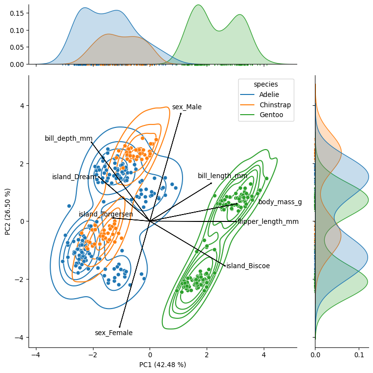
g = sns.jointplot(data=pca_data, x="PC1", y="PC2", hue="species", ratio=4, marginal_ticks=True, height=8)
g.plot_joint(sns.kdeplot, zorder=0, levels=6)
g.plot_marginals(sns.rugplot, height=-.025, clip_on=False)
# Add loadings
loading_plot(loadings[["PC1", "PC2"]].values, loadings.index, text_x=text_x, text_y=text_y, scale=2, arrow_size=0.02)
# Add variance explained by the
plt.xlabel(f"PC1 ({pca_step.explained_variance_ratio_[0]*100:.2f} %)")
plt.ylabel(f"PC2 ({pca_step.explained_variance_ratio_[1]*100:.2f} %)")
plt.tight_layout()
plt.savefig("PCA_with_loadings.png", dpi=300)
plt.show()/var/folders/mn/wpqfzxsn0z10p73_8jr0v2180000gn/T/ipykernel_56853/3221505183.py:36: FutureWarning: Series.__getitem__ treating keys as positions is deprecated. In a future version, integer keys will always be treated as labels (consistent with DataFrame behavior). To access a value by position, use `ser.iloc[pos]`
text_x[i] if text_x.all() else coeff[i, 0] * 1.2 * scale,
/var/folders/mn/wpqfzxsn0z10p73_8jr0v2180000gn/T/ipykernel_56853/3221505183.py:37: FutureWarning: Series.__getitem__ treating keys as positions is deprecated. In a future version, integer keys will always be treated as labels (consistent with DataFrame behavior). To access a value by position, use `ser.iloc[pos]`
text_y[i] if text_y.all() else coeff[i, 1] * 1.2 * scale,Text(0.5, 55.813333333333325, 'PC1 (42.48 %)')Text(60.083333333333336, 0.5, 'PC2 (26.50 %)')sns.displot(df, x="bill_length_mm", kde=True, rug=True, hue="species", stat="proportion");
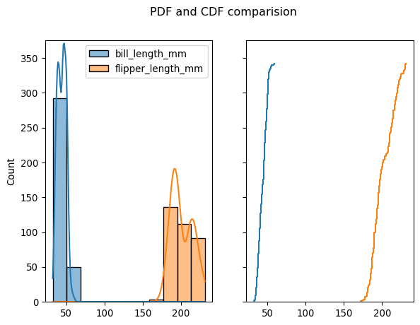
plt.show()fig, axes = plt.subplots(1, 2, sharey=True)
fig.suptitle('PDF and CDF comparision')
sns.histplot(df[["bill_length_mm", "flipper_length_mm"]], kde=True, ax=axes[0]);
sns.ecdfplot(df[["bill_length_mm", "flipper_length_mm"]], stat="count", ax=axes[1], legend=False)
plt.ylim((0, 375));
plt.show()Text(0.5, 0.98, 'PDF and CDF comparision')import pathliblr = LogisticRegression(max_iter=10000)
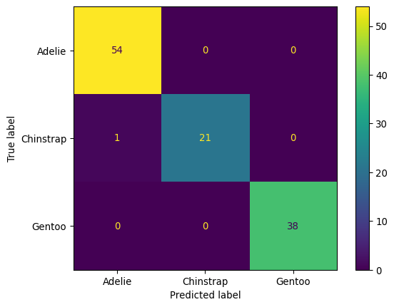
X_train, X_test, y_train, y_test = train_test_split(X, y, test_size=0.33, random_state=42)
lr.fit(X_train, y_train)
cmd = ConfusionMatrixDisplay.from_estimator(lr, X_test, y_test)
plt.show()LogisticRegression(max_iter=10000)In a Jupyter environment, please rerun this cell to show the HTML representation or trust the notebook.
On GitHub, the HTML representation is unable to render, please try loading this page with nbviewer.org.
Parameters
| penalty | 'l2' | |
| dual | False | |
| tol | 0.0001 | |
| C | 1.0 | |
| fit_intercept | True | |
| intercept_scaling | 1 | |
| class_weight | None | |
| random_state | None | |
| solver | 'lbfgs' | |
| max_iter | 10000 | |
| multi_class | 'deprecated' | |
| verbose | 0 | |
| warm_start | False | |
| n_jobs | None | |
| l1_ratio | None |
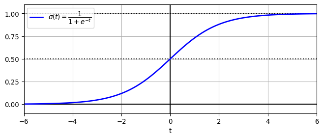
Logistic function visualization
# https://github.com/ageron/handson-ml3/blob/main/04_training_linear_models.ipynb
lim = 6
t = np.linspace(-lim, lim, 100)
sig = 1 / (1 + np.exp(-t))

plt.figure(figsize=(8, 3))
plt.plot([-lim, lim], [0, 0], "k-")
plt.plot([-lim, lim], [0.5, 0.5], "k:")
plt.plot([-lim, lim], [1, 1], "k:")
plt.plot([0, 0], [-1.1, 1.1], "k-")
plt.plot(t, sig, "b-", linewidth=2, label=r"$\sigma(t) = \dfrac{1}{1 + e^{-t}}$")
plt.xlabel("t")
plt.legend(loc="upper left")
plt.axis([-lim, lim, -0.1, 1.1])
plt.gca().set_yticks([0, 0.25, 0.5, 0.75, 1])
plt.grid()
plt.show()
Text(0.5, 0, 't')Obtain the logistic function mathematically
Step 1. Write out the linear regression equation
\(\Huge y=\beta_0+\beta_1 x_1+...+\beta_n x_n\) ## Step 2. The logistic regression equation is the same as above except output is log odds \(\Huge log(odds)=\beta_0+\beta_1 x_1+...+\beta_n x_n\) ## Step 3. Exponentiate both sides of the logistic regression equation to get odds \(\Huge odds=e^{\beta_0+\beta_1 x_1+...+\beta_n x_n}\) ## Step 4. Write out the probability equation \(\Huge p=\frac{odds}{1+odds}\) ## Step 5. Plug odds (from step 3) into the probability equation \(\Huge p=\frac{e^{\beta_0+\beta_1 x_1+...+\beta_n x_n}}{1+e^{\beta_0+\beta_1 x_1+...+\beta_n x_n}}\) ## Step 6. Divide the numerator and denominator by the odds (from step 3) \(\Huge p=\frac{1}{1+e^{-(\beta_0+\beta_1 x_1+...+\beta_n x_n)}}\)
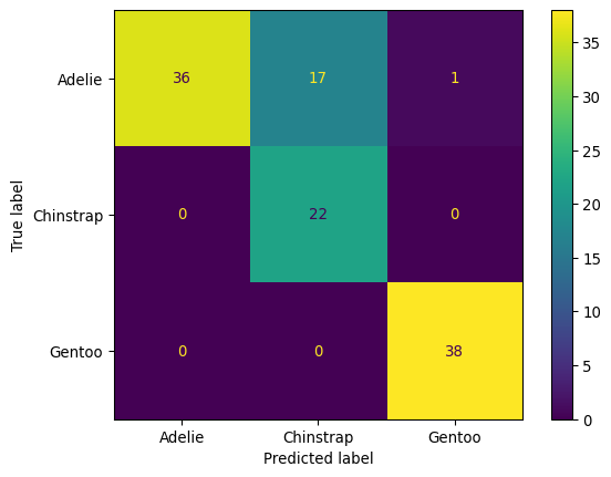
gnb = GaussianNB()
gnb.fit(X_train, y_train)
cmd = ConfusionMatrixDisplay.from_estimator(gnb, X_test, y_test)
plt.show()GaussianNB()In a Jupyter environment, please rerun this cell to show the HTML representation or trust the notebook.
On GitHub, the HTML representation is unable to render, please try loading this page with nbviewer.org.
Parameters
| priors | None | |
| var_smoothing | 1e-09 |
ct = pd.crosstab(df["species"], df["body_mass_g"] > df["body_mass_g"].mean(), margins=True)ct| body_mass_g | False | True | All |
|---|---|---|---|
| species | |||
| Adelie | 127 | 25 | 152 |
| Chinstrap | 61 | 7 | 68 |
| Gentoo | 7 | 117 | 124 |
| All | 195 | 149 | 344 |
likelihood = ct.iloc[0, 0] / ct.iloc[0, 2]
likelihoodnp.float64(0.8355263157894737)prior = ct.iloc[0, 2] / ct.iloc[3, 2]
priornp.float64(0.4418604651162791)norm = ct.iloc[3, 0] / ct.iloc[3, 2]
normnp.float64(0.5668604651162791)posterior = ct.iloc[0, 0] / ct.iloc[3, 0]
posteriornp.float64(0.6512820512820513)\(\Huge P(A\vert B)={\frac {P(B\vert A)P(A)}{P(B)}}\)
result = likelihood * prior / normdf["body_mass_g"] > df["body_mass_g"].mean()0 False
1 False
2 False
3 False
4 False
...
339 False
340 True
341 True
342 True
343 True
Name: body_mass_g, Length: 344, dtype: bool# gnb.fit([df["body_mass_g"] > df["body_mass_g"].mean()], y)Citation
@online{laptev2024,
  author = {Laptev, Martin},
  title = {Probability},
  date = {2024},
  urldate = {2024},
  url = {https://maptv.github.io/ml/prob/},
  langid = {en}
}
